Introduction

Estimates of daily infections are the critical input into the COVID-19 forecast (SEIR) model. Many early models assumed that cases equaled infections or that the infection-detection rate (IDR) was constant over time and across locations. Early scarcity of PCR testing for COVID-19 was followed by rapid expansion of testing capacity in many high-income countries, while many low-resource settings continue to have low testing rates, all suggesting substantial variation in IDR over time and across locations. Until January 2021, the IHME model used deaths, a metric that has been less affected by PCR testing availability, to estimate infections using empirical estimates of the infection-fatality ratio (IFR). Estimates of the IFR based on seroprevalence surveys matched to deaths vary over time and location. Starting with the January 22 release of our COVID-19 forecast model, we adopted an approach that maps cases to infections, hospitalizations to infections, and deaths to infections, and then generates the composite estimate of past infections from these three series. Since then, we have made further improvements to this model. Specifically, we now take into account the effect of waning immunity on seroprevalence surveys and introduce a more robust method for predicting the IDR, infection-hospitalization rate (IHR), and IFR in settings without seroprevalence surveys. These model updates are included in the April 23 release of our estimates. This document provides more detail on the statistical models used in this approach.

Overview

Our approach has six distinct components. First, we address missingness and reporting anomalies present in COVID-19 statistics that get reported on a daily basis. Second, we adjust seroprevalence surveys for vaccination rates, re-infection from escape variants (Beta and Gamma), and antibody test sensitivity and waning. Third, we produce empirical estimates of the IDR, IHR, and IFR by using corrected cumulative infections, which are derived from representative seroprevalence surveys paired with cumulative cases, cumulative hospitalizations, and cumulative deaths. We have developed statistical models to project the IDR, IHR, and IFR for each location and day. Fourth, we generate a smooth curve of daily cases, daily hospitalizations (where available), and daily deaths using splines. Fifth, we generate three time series of estimated past daily infections by dividing the time series of cases, hospitalizations, and deaths by the IDR, IHR, and IFR, respectively. We then combine all three of these series into a single composite estimate of the time trend of infections from the beginning of the pandemic to now. Sixth, we use daily infections to estimate the cumulative percentage of individuals with one or more infections, which we then compare to seroprevalence surveys to assess the internal consistency in each step of our modeling process.

1. Input data corrections

We make several types of corrections to reported data to take into account common challenges that have emerged during the course of the pandemic. First, for some locations, hospital time series do not have complete time coverage. We impute the missing part of the hospital series using the relationship between hospitalizations and cases and deaths. 

Second, we track lags in the reporting for cases, hospitalizations, and deaths for each location. Figure 1 shows an example of this type of analysis. It shows the number of deaths reported by day by the Washington State Department of Health for five weeks in a row at one-week intervals. The figure clearly shows significant reporting lags that could easily lead to incorrect inference about the trend in infections. Including data with reporting lags can lead to false estimates of declining transmission in SEIR models. 

To avoid that, in locations where we identify major reporting lags, we drop the more recently reported data from the analysis. We have found that reporting lags differ by location and for cases, hospitalizations, and deaths.

Figure 1: Daily deaths as reported by the Washington State Department of Health over five weeks from February 1 to March 1, 2021. This figure demonstrates that there is substantial underreporting over the last 10 days for each series.

 

2. Adjusting seroprevalence data for vaccination, re-infection due to escape variants, and declining antibody test sensitivity as a function of time since infection

Vaccination generates a positive anti-spike antibody test in nearly all individuals with an immune response to the vaccine. The impact of vaccination on seroprevalence is clear in some settings with rapid scale-up of vaccination, such as England. To account for this, we adjust the seroprevalence estimates downward to consider vaccination rates in adults using the following equation: 

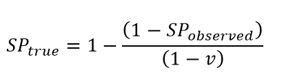
where SP_true is true seroprevalence, SP_observed is observed seroprevalence, and v is the vaccination rate.

In settings with escape variants present, seroprevalence surveys provide an estimate of the cumulative number of individuals with one or more infections. To compute the IFR, IHR, and IDR, we need an estimate of cumulative infections, including re-infections. We estimate the number of cumulative infections from seroprevalence surveys, based on the prevalence of escape variants (Beta and Gamma) and an assumed level of cross-variant immunity of 30% between the escape variants, ancestral variants, and other variants, such as Alpha, that do not show immune escape. This estimate is derived from an empirical analysis using our SEIR model of the scale-up of Gamma in Amazonas, Brazil, and Beta in South Africa. For this stage of our analysis, we approximate the time pattern of past infection based on using deaths divided by a preliminary estimate of the infection-fatality rate (see below) – we will later use the adjusted seroprevalence to re-estimate the IFR. The formula for the correction for escape variant prevalence is:

where cumulative ancestral-type infections at time t, , is a function of daily observed infections, , and daily escape variant prevalence, ; unprotected population fraction at time t, U_t, is the percentage of individuals exposed to ancestral-strain COVID not protected by cross-variant immunity, c; and ancestral-type infections re-infected with escape-variant COVID at time t, , is then the product of unprotected exposed, observed infections, and escape variant prevalence. The adjustment scalar at time t, s_t, is then applied to seroprevalence data in order to account for repeat infections.

Published studies following cohorts of patients with positive viral tests show declining antibody test sensitivity as a function of time since infection (further detail here, here, and here). These studies suggest that anti-nucleocapsid tests generally perform worse than anti-spike tests over time. Within each class, different commercial tests also have different rates of declining sensitivity. To adjust each reported seroprevalence survey, we use information on the specific test used in each survey, the pattern of declining sensitivity over time, and information on the time pattern of infections. We once again use a preliminary estimate of infections based on the IFR. For each seroprevalence observation, we determine how many past infections would have tested positive based on the number of days between exposure and midpoint of the study dates in the serology study and the antibody test used. We use the ratio of total estimated infections to the cumulative sum of presumed positives to adjust the seroprevalence data.   

The estimates of cumulative infection that result from these processes are then used in a more robust estimation of IFR, IDR, and IHR.

3. Modeling deaths, hospitalizations, and confirmed cases per infection

3a. Bayesian regression cascade

Models for IFR, IHR, and IDR are fit using MRTool, an open-source Bayesian meta-regression library developed at IHME. We have implemented a “cascading” framework wherein after a global model is fit using all available data, subsequent models are fit using only data pertaining to subsets of a geographic hierarchy with levels for super-region, region, country, and subnational (where possible). We use an adapted version of the Global Burden of Disease location hierarchy in this algorithm. In each of these models, the mean and standard deviation of the coefficients estimated in the “parent” location model are passed on to “child” location models as Gaussian priors. For example, a model for the high-income super-region is fit using data from all locations within that super-region, and is also informed by all available data through the priors that are derived from the global model coefficients. Similarly, a model for Western Europe uses data directly from countries within that region and is also informed by the high-income model through the priors. Taking this a step further down the “cascade,” the model for Belgium uses only country-specific data and is also informed by the Western European parent model through the priors that it uses. Locations without seroprevalence data use the parameters estimated from the model of the nearest parent location for prediction.

3b. Estimating the infection-fatality rate

Using seroprevalence surveys where we can match to deaths due to COVID-19, we have obtained 1,181 direct measurements of the infection-fatality ratio (IFR). Because age is such an important determinant of the IFR, we first analyze the age pattern of the IFR and use that to analyze the broader set of all-age IFR measurements using indirect age-standardization methods.

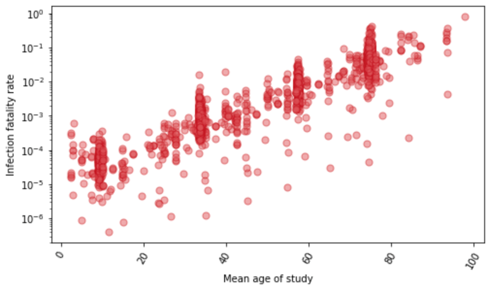
For a subset of locations with age-specific data on seroprevalence and reported COVID-19 deaths, we estimate the age-specific IFR directly. Figure 2 shows the relationship between IFR and age for these 1,879 data points. We find that the IFR generally increases nearly 10% for each year of age. At the youngest ages, the relationship appears to be J-shaped, where the IFR decreases from age 0 to 10 and then starts increasing steadily with each year of age. Because of the strong relationship with age, we use age-standardized IFR data in subsequent all-age analyses. Because many seroprevalence surveys only provide all-age seroprevalence, we use indirect standardization methods to generate age-standardized rates. Indirect standardization computes the ratio of observed IFR to the IFR that is expected based on each location’s population age structure and the global age pattern of the IFR.   

Figure 2: The relationship between Infection-fatality rate and age, based on 1,879 measurements of IFR. These measurements are derived from pairing age-specific seroprevalence results and COVID-19 deaths by age. Y-axis is shown in log base 10.

 

Patient-level data from registries of US hospital patients, US claims data, and Brazil hospitalizations for COVID-19 all show that the hospital-fatality rate decreased from March 2020 through to late fall and then increased in many settings. The increase in the hospital-fatality rate may have been due to changes in the tendency to admit moderately severely ill patients to hospital when there was more demand on available hospital beds. These patient-level studies on the hospital-fatality rate strongly suggest that the prevalence of obesity is an important predictor of the hospital-fatality rate. 

We estimate the logit-transformed age-standardized IFR as a function of time and age-standardized obesity by location. The age-standardization is then reversed when predicting out from the model. Time indexing of IFR data is based on the average date of death for each observation. We use the patient-level data on the hospital-fatality rate to inform the prior on the obesity coefficient. We also incorporate the conclusion from that analysis that the IFR was declining from March until sometime in the summer or fall – for each location, we tested if the IFR stopped declining in each month from May to November by running separate linear spline regressions with one knot fixed to the first day of each of those months, where the IFR is allowed to decline in the period preceding the knot and is held constant following that date. We select the date of inflection for each location based on the best fit to seroprevalence data in the nearest location in the geographic hierarchy with at least one observation later than July 1, 2020, in order to ensure that evaluation is informed by data beyond the nascent stages of the pandemic. Lastly, we account for changes in the all-age IFR caused by differential vaccination rates by age, as well as the presence of more lethal variants.

Figure 3: Observed and predicted infection-fatality rate over time for Georgia, United States

3c. Infection-detection rate

We have identified 1,181 seroprevalence surveys that are representative of the general population in the settings where they were conducted or sampled from populations that can be considered representative, such as blood donors. For each survey, the seroprevalence estimates adjusted for vaccination, waning antibody sensitivity, and re-infection rates are used to estimate cumulative infections. These are then matched with cumulative reported cases to generate an empirical estimate of the average infection-detection rate over the interval from the beginning of the pandemic to the date of the seroprevalence survey data collection. For the calculation of the IDR, the appropriate lags have been used to match cumulative infections estimated from the seroprevalence survey to cumulative cases to reflect both the average time from infection to getting diagnosed as a case and the lag between infection and becoming antibody-positive. Figure 4 shows all the estimates of the IDR against time. The estimate of the IDR is time-localized to the average date of infection based on the model estimate and daily cases. 

Figure 4: Empirical measurements of the infection-detection rate based on 1,181 paired seroprevalence surveys and reported cases plotted against time

We evaluated a number of covariates to predict the IDR (modeled as logit IDR). In the model, we use the log of the infection-weighted average testing capacity at the time of the surveillance observation, where testing capacity is defined as the maximum testing rate at a given date. We then predict the daily IDR using the observed daily testing capacity. Figure 5 shows the data on IDR for the state of Georgia, USA, and the predictions from the model. The observed IDR increased during the course of the pandemic. Because even in the beginning of the pandemic when testing rates were low, severely ill patients would have gone to hospital and many would have been diagnosed, we set location-specific floor values for the IDR. To estimate the value for the floor, we use an iterative selection algorithm that tests values between 0.01% and 10% and selects the value that yields the best fit to the available seroprevalence data. 

Figure 5: Observed and predicted infection-detection rate over time for Georgia, United States

 

3d. Infection-hospitalization rate

By matching seroprevalence surveys to cumulative hospitalizations, we get 1,033 direct measurements of the infection-hospitalization rate (IHR). For a subset of locations with age-specific data on seroprevalence and hospitalizations, we have direct measurements of age-specific IHR. Figure 6 shows these 1,750 data points against age. There is a marked relationship where the IHR generally increases nearly 5% per each single year of age. Because of the strong relationship with age, we use age-standardized IHR data in subsequent modeling steps. Many seroprevalence surveys only provide estimates of all-age seroprevalence, so we have used indirect standardization methods to generate age-standardized rates.

Figure 6: Infection-hospitalization rate observations (N=1,750) as a function of age based on paired age-specific seroprevalence results and COVID-19 hospitalizations by age. Plot is shown in log base 10.

 

Figure 7 shows the relationship for age-standardized IHR measurements and time; there is considerable between-location variation but, unlike the IDR, not an obvious time trend.

Figure 7: Age-standardized infection-hospitalization rate based on 1,033 seroprevalence surveys paired with cumulative hospitalizations plotted against time. Y-axis is shown in log base 10.

 

We explored several covariates, including the prevalence of obesity and other comorbidities, but did not find any predictive relationships, so we use an intercept-only model to estimate logit age-standardized IHR. The predicted age-standardized IHR for each location is then converted to an estimate of the all-age IHR that reflects local population age structure, reversing the procedure for indirect age-standardization. As with the IFR, we account for changes in the all-age IHR caused by differential vaccination rates by age and the presence of escape variants.

4. Smoothed time series of cases, hospitalizations, and deaths

Reporting patterns for cases and deaths exhibit substantial variation according to the day of the week. We also observe characteristic patterns of lagged and then catch-up reporting around holiday periods – notably Thanksgiving in the USA, the last week of December, and Easter. We fit a smooth function to these in two steps. First, we prime the smoother by taking a centered seven-day rolling average of each daily reported measure, allowing every data point to be informed by reporting from each day of the week. We then fit a cubic spline to the natural log of those data with a knot every seven days. Figure 8 shows for Georgia, USA, the daily reported cases, hospitalizations, and deaths, as well as the output of the smoother.

Figure 8: Observed and smoothed daily cases, hospitalizations, and deaths for Georgia, United States

 

5. Daily infections

For each smoothed time series of cases, hospitalizations, and deaths, we generate an estimate of daily infections by dividing by the IDR, IHR, and IFR, respectively. Each estimated sequence of daily infections is shifted in time to take into account the natural history from infection to case identification, hospitalization, and death. Specifically, we assume that on average the time from infection to becoming a diagnosed case is 11 days, for a hospitalization it is 11 days, and for death it is 24 days. There may be variation in the lag between infection and various outcomes across locations and over time, but in this analysis we assume these lags do not vary.

The approach we use to combine the series into a single composite estimate of daily infections is designed to deal with the compositional bias problem caused by varying temporal coverage among cases, hospitalizations, and deaths, or due to different lags in the time between infection and those events. The unit of the analysis in the initial stage of synthesizing these measures is the first difference in log daily values. We incorporate these data into a random knots spline regression using MRTool without the cascading framework, wherein we provide a number of knots and a number of unique knot combinations to an algorithm that runs a model with each combination and makes a weighted composite estimate from the sub-models based on in-sample performance. We specify one knot per 28 days of data, and test 100 random knot combinations of a quadratic spline. We then convert the estimate into ln(daily) values by taking the cumulative sum and find the initial value of the composite time series by fitting a model to the average ln(daily) residual of the three original curves with respect to the composite.

Figure 9: Daily infections for Georgia, United States, as a function of deaths, hospitalizations, and cases, as well as a composite estimate of infections based on those data

 

In order to incorporate uncertainty in our infections estimate based on the consistency of our three inputs, as well as measurement error in those data, we perform additional steps to create samples of our infections curve reflective of that error. We first convert the observed daily cases, hospitalizations, and deaths into “observed” infections by dividing them by the estimated time series of IDR, IHR, and IFR, respectively. We then use the log of these values to compute the residuals with respect to the mean infections curve we have estimated in the previous step and calculate the robust standard deviation. With that, we independently sample 1,000 infections for each day, which gives us 1,000 uncorrelated time series of ln(daily infections) that are representative of the noise in the raw data. We then refit curves to these noisy series using our random knots spline model; in this step, we use a cubic spline based on one randomly sampled knot combination per time series draw, again based on one knot per 28 days of data, to produce 1,000 smooth past infections curves.

6. Comparison of cumulative infections to seroprevalence surveys

The last part of the model diagnostics, shown in Figure 10, is a comparison of cumulative infections from the series based on cases divided by the IDR, hospitalizations divided by the IHR, and deaths divided by the IFR, along with the pooled composite estimate. We also plot on this diagram available seroprevalence surveys, which allows for visual assessment of the consistency between the various approaches. These plots can be useful in identifying where there are major disconnects in the time series. 

Figure 10: Cumulative infection rate for Georgia, United States, as a function of deaths, hospitalizations, and cases, as well as a composite estimate of infection rate with uncertainty based on those data. Also plotted are seroprevalence survey data.