Background and data

The Institute for Health Metrics and Evaluation (IHME) has produced estimates of the extreme poverty counts and rates from 1990 to 2050. Extreme poverty rate (hereafter referred to as poverty rate) is defined as the fraction of the population living at or below $1.90 per day, measured using 2011 purchasing-power parity-adjusted dollars. These estimates rely on data extracted from the World Bank World Development Indicators database and the Financing Global Health database as the primary sources of data (1–3). For both retrospective and prospective estimates, poverty rates were modeled. Poverty counts were calculated by multiplying the poverty rates by the population (4). Table 1 identifies all data and data sources used in this study.

Table 1: Data sources

Data series	Units	Data source
Extreme poverty rate	Fraction of the population living at or below $1.90 per day, measured using 2011 purchasing-power parity-adjusted dollars	World Bank World Development Indicators (3)
Gross domestic product	Monetary value of all the finished goods and services produced within a country’s borders in a specific time period, measured using 2011 purchasing-power parity-adjusted dollars	IHME (5)
Mortality rate due to shocks	Deaths due to military operations, terrorism, natural disasters, or famine. Measured in per capita terms	IHME (6)
Energy consumption	Amount of energy that a person needs to carry out a physical function such as breathing, circulating blood, digesting food, or physical movement	IHME (7)
Female Educational attainment	Mean years of education obtained for females age 15 to 19	IHME (8)
Total fertility rate	Total number of births per 1,000 women	IHME (6)
General government expenditure	All government current expenditures for purchases of goods and services (including compensation of employees) as a fraction of the country’s GDP	IHME (1,2)

Methods

Retrospective estimates

IHME extracted poverty rate data from the World Bank World Development Indicators (3). These data include 1,457 country-years of data between 1980 and 2018. Table 2 identifies the countries and the number of years with reported poverty data extracted from the World Bank World Development Indicators Database. In order to generate a complete and consistent time-series, we used spatiotemporal Gaussian process regression (ST-GPR), a Bayesian method used in the Global Burden of Disease (GBD) study, to estimate poverty rates in 195 countries from 1980 through 2017 (10). ST-GPR is a three step modeling process. First, a linear mixed effects model was run with a set of predictive covariates (GDP per capita, female education, and energy consumption, see Table #1). Predictions from the first step provide the general trend within the data. In the second step, spatiotemporal patterns were estimated by applying a series of spatiotemporal weights to average the residuals of the first step linear model. These spatiotemporal patterns were then added to the linear prediction to generate spatiotemproal predictions. Finally, the spatiotemporal predictions served as the mean function of a Gaussian process regressions run across time on the data. Estimates from the Gaussian process regressions served as final ST-GPR predictions and generated a complete time-series of estimates from 1990 to 2017 in 195 countries, building from data when available and borrowing strength across time, geography, and covariates’ predictive power when data was not available.

Table 2: Countries included in this study

Country	Years of Data
Albania	5
Algeria	3
Angola	2
Argentina	29
Armenia	18
Australia	10
Austria	13
Azerbaijan	6
Bangladesh	9
Belarus	20
Belgium	13
Belize	6
Benin	3
Bhutan	4
Bolivia	19
Bosnia and Herzegovina	4
Botswana	5
Brazil	33
Bulgaria	10
Burkina Faso	5
Burundi	4
Cameroon	4
Canada	11
Cape Verde	2
Central African Republic	3
Chad	2
Chile	14
China	13
Colombia	19
Comoros	2
Congo	2
Costa Rica	31
Cote d'Ivoire	10
Croatia	8
Cyprus	12
Czech Republic	14
Democratic Republic of the Congo	2
Denmark	13
Djibouti	4
Dominican Republic	22
Ecuador	20
Egypt	8
El Salvador	24
Estonia	14
Ethiopia	5
Fiji	3
Finland	13
France	13
Gabon	2
Georgia	22
Germany	18
Ghana	7
Greece	13
Guatemala	6
Guinea	5
Guinea-Bissau	4
Guyana	2
Haiti	1
Honduras	28
Hungary	15
Iceland	12
India	6
Indonesia	25
Iran	11
Iraq	2
Ireland	13
Israel	10
Italy	13
Jamaica	7
Japan	1
Jordan	7
Kazakhstan	18
Kenya	5
Kiribati	1
Kyrgyzstan	19
Laos	5
Latvia	15
Lebanon	1
Lesotho	4
Liberia	3
Lithuania	13
Luxembourg	13
Madagascar	8
Malawi	4
Malaysia	12
Maldives	2
Mali	4
Malta	10
Mauritania	7
Mauritius	2
Mexico	15
Moldova	21
Mongolia	9
Montenegro	10
Morocco	6
Mozambique	4
Myanmar	1
Namibia	3
Nepal	3
Netherlands	12
Nicaragua	6
Niger	6
Nigeria	5
Norway	13
Pakistan	12
Panama	24
Papua New Guinea	2
Paraguay	21
Peru	21
Philippines	11
Poland	21
Portugal	13
Romania	13
Russian Federation	21
Rwanda	6
Samoa	3
Sao Tome and Principe	2
Senegal	5
Serbia	11
Seychelles	1
Sierra Leone	3
Slovakia	13
Slovenia	13
Solomon Islands	2
South Africa	7
South Korea	4
South Sudan	1
Spain	13
Sri Lanka	8
Sudan	1
Suriname	1
Swaziland	3
Sweden	13
Switzerland	10
Syria	1
Tajikistan	6
Tanzania	4
Thailand	23
The Gambia	4
Timor-Leste	3
Togo	3
Tonga	3
Trinidad and Tobago	2
Tunisia	7
Turkey	17
Turkmenistan	1
Uganda	9
Ukraine	19
United Kingdom	12
United States	10
Uruguay	14
Uzbekistan	4
Vanuatu	1
Venezuela	13
Vietnam	10
Yemen	3
Zambia	9
Zimbabwe	1

Prospective estimates

We forecasted the number of people living in poverty from 2018 through 2050 by estimating the year-over-year change in the poverty rates using an ensemble forecasting model approach (2). Instead of relying on a single model, the ensemble forecasting considers a large set of possible combinations of mixed effects models to generate long-term forecasts.

Covariates considered in the ensemble were GDP per capita, maternal educational attainment per capita, total fertility rate, and general government expenditure measured as a share of the gross domestic product. These covariates were used for the ensemble because forecasts of these covariates through 2050 exist (2,4). We required GDP per capita to be included in each sub-model of the ensemble. The ensemble also considered a number of additional time-series modeling factors. We incorporated up to three degrees of autoregression, where the coefficients were varied at both global and country-specific levels. We also considered the inclusion of a convergence term, which is a single-year lag of the level valued dependent variable. We incorporated four distinct weighting schemes to allow for potential up-weighting of recent time-trends. Finally, we included country-specific random intercepts for all sub-models to capture country-specific heterogeneity.

Table 3: Coefficients of selected covariates used in the ensemble forecasts

Covariate	Minimum	Mean	Maximum
Gross domestic product	-0.914	-0.628	-0.003
General government expenditure	-0.020	-0.015	-0.008
Maternal educational attainment	-0.074	-0.074	-0.073
Total fertility rate	-	-	-

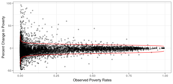
We ran a total of 448 sub-models, which includes all combinations of the covariates and other forecasting components. All of the 448 sub-models were evaluated based on a set of three inclusion criteria: (i) all of the estimated coefficients had to have at least a 90% level of statistical significance (p-value < 0.1); (ii) the estimated coefficients must not defy imposed prior assumptions (e.g., we dropped all models where the coefficient on GDP per capita was positive, since we do not believe that the marginal correlation between poverty and GDP per capita is positive); and (iii) the future poverty rate time trends must not exceed extreme growth. We defined extreme growth rates using a frontier model fit on retrospective poverty rate data, such that year-over-year changes in poverty rates were constrained relative to the country’s poverty rate. Figure 1 illustrates the observed year-over-year poverty rate changes and the frontier.

Figure 1: Defining extreme year-over-year poverty rate changes

Once we filtered out and retained the “best” sub-models, we held out 10 years of recent data (2008–2017) and used the retained sub-models to forecast those years of poverty rates. The difference of the observed and forecasted poverty rates between 2008 through 2017 were used to evaluate out-of-sample predictive validity, using root mean squared errors (RMSE). The ensemble model included 10% of the remaining sub-models with lowest RMSE for each country-year. We simulated 1,000 draws of the future across the remaining sub-models to create the final set of poverty rate forecasts between 2018 and 2050.

Alternative future poverty scenarios

In addition to the reference future scenario of poverty (described above), we generated better and worse scenarios of poverty to identify how our reference future poverty scenarios would change with alternative covariate scenarios (9). We developed better and worse scenarios by adjusting each of the covariates used in our reference model in the following ways.

Gross domestic product: The alternative GDP per capita scenarios highlight how GDP per capita would change with alternative annual growth rates.

General government expenditure: The fraction of GDP that was general government expenditure was held constant across our alternative scenarios.

Maternal educational attainment: In order to estimate future HCI scenarios, future better and worse education scenarios were created (9). Those better and worse education scenarios replace country-specific growth in education attainment with growth associated with the 85^th and 15^thpercentiles of weighted annualized rates of change of educational attainment per capita across the 195 countries observed in retrospective data.

Total fertility rate: The reference scenario of age-specific fertility rate (ASFR) for all age groups were forecasted using reference education and reference contraceptive met need as covariates. In order to generate the better and worse scenarios of ASFR, better and worse scenarios of educational attainment discussed above were used, rather than the reference education scenarios. Met need of contraceptive was held the same at the reference scenario. Total fertility was computed using ASFR. More details on the models used for forecasting ASFR are explained in Foreman et al (4).

References

1. Dieleman JL, Haakenstad A, Micah A, Moses M, Abbafati C, Acharya P, et al. Spending on health and HIV/AIDS: domestic health spending and development assistance in 188 countries, 1995--2015. Lancet. 2018;391(10132):1799–829.

2. Dieleman JL, Sadat N, Chang AY, Fullman N, Abbafati C, Acharya P, et al. Trends in future health financing and coverage: future health spending and universal health coverage in 188 countries, 2016–40. Lancet. 2018;

3. World Bank. World Development Indicators | DataBank [Internet]. [cited 2018 Sep 13]. Available from: http://databank.worldbank.org/data/source/world-development-indicators#

4. Foreman KJ, Marquez N, Dolgert A, Fukutaki K, McGaughey M, Pletcher MA, et al. Forecasting life expectancy, years of life lost, all-cause and cause-specific mortality for 250 causes of death: reference and alternative scenarios 2016–2040 for 195 countries and territories. Lancet. 2018;

5. James SL, Gubbins P, Murray CJL, Gakidou E. Developing a comprehensive time series of GDP per capita for 210 countries from 1950 to 2015. Popul Health Metr. 2012 Jul;10(1):12.

6. Abajobir AA, Abate KH, Abbafati C, Abbas KM, Abd-Allah F, Abera SF, et al. Global, regional, and national under-5 mortality, adult mortality, age-specific mortality, and life expectancy, 1970–2016: a systematic analysis for the Global Burden of Disease Study 2016. Lancet. 2017;390(10100).

7. Schmidhuber J, Sur P, Fay K, Huntley B, Salama J, Lee A, et al. The Global Nutrient Database: availability of macronutrients and micronutrients in 195 countries from 1980 to 2013. Lancet Planet Heal [Internet]. 2018 Aug 1 [cited 2018 Sep 13];2(8):e353–68. Available from: http://www.ncbi.nlm.nih.gov/pubmed/30082050

8. Gakidou E, Cowling K, Lozano R, Murray CJL. Increased educational attainment and its effect on child mortality in 175 countries between 1970 and 2009: a systematic analysis. Lancet. 2010;376(9745):959–74.

9. Lim SS, Updike R, Kaldijan A, Barber R, Cowling K, York H, et al. Measuring human capital: a systematic analysis of 195 countries and territories, 1990–2016. Forthcoming. 2018;

10. Abajobir AA, Abate KH, Abbafati C, Abbas KM, Abd-Allah F, Abdulle AM, et al. Global, regional, and national comparative risk assessment of 84 behavioural, environmental and occupational, and metabolic risks or clusters of risks, 1990–2016: a systematic analysis for the Global Burden of Disease Study 2016. Lancet. 2017;390(10100).

11. Hoeting JA, Madigan D, Raftery AE, Volinsky CT. Bayesian model averaging: a tutorial. Stat Sci. 1999;382–401.

12. Zeugner S, Feldkircher M. Bayesian Model Averaging Employing Fixed and Flexible Priors: The {BMS} Package for {R}. J Stat Softw. 2015;68(4):1–37.

Methods for estimating past and future extreme poverty